As observability becomes a foundational layer in modern enterprise IT, the challenge is no longer the lack of data — but what to do with it. Metrics, logs, and events stream in by the millions. What teams need is a way to understand when system behavior begins to shift — whether suddenly or silently — and whether that shift demands attention.
Anomaly detection helps surface these changes. However, an anomaly manifests in many different forms. Some issues appear as sharp spikes while others creep in over time. Some show up only when multiple metrics are considered together. And many don’t look anomalous at all — until someone connects the dots across layers.
Let’s walk through how anomalies manifest in IT systems, why simple threshold-based detection isn’t enough, and how modern detection methods adapt to increasingly complex environments.
Detecting sudden spikes: point-in-time anomaly
Point-in-time anomalies are among the most intuitive types of deviations observed in enterprise systems. These are sudden spikes or drops in a metric — such as CPU utilization, memory consumption, response time, or error rates — that stand out from normal behavior at a specific moment.
Because they appear sharp and visible, they are often treated as the most “obvious” anomalies. However, reliably detecting them in a production environment is rarely straightforward.
Most systems begin with static thresholds — rules such as “raise an alert if application response time exceeds 2 seconds.” While easy to configure, such rules often lead to noise. They ignore system-specific baselines and don’t adapt to known patterns such as backup schedules or housekeeping activities, or peak usage windows. As a result, they either trigger too often or fail to raise alerts when something truly unusual occurs just below the threshold.
In real-world IT environments, business and technical changes are constant. Several factors bring the change, whether it’s new hardware, a patch installation, application onboarding, or seasonal events like sales or promotions. These factors can shift what “normal” looks like for your system, requiring the baseline for detection to be updated accordingly.
To adapt, the first step is to identify when a meaningful and persistent change in behavior has occurred. Various change detection algorithms can help pinpoint these transitions in the data, separating temporary fluctuations from true shifts. Once a new steady state is established, you can then derive thresholds that reflect the most recent, stable behavior of the system.
Even within a steady state, a single threshold rarely captures all patterns of normal behavior. For example, systems often behave differently on weekdays versus weekends, or during day and night hours. Recognizing these temporal patterns is key — by identifying and segmenting these regular cycles, you can apply separate thresholds that better reflect the expected behavior in each period. This approach helps manage recurring patterns, seasonality, and operational noise, so that alerts remain meaningful and actionable rather than overwhelming.
To manage noise and ensure relevance, detection sensitivity can be tuned based on the business context. For example, a moderate deviation might raise a minor warning, while a larger deviation could trigger a critical alert. This also allows teams to adjust the aggressiveness of detection in different modes. Some false positives may be tolerated in anomaly-detection mode, or a more proactive mode that surfaces early signals at the risk of some false alarms. This flexibility ensures that alerts are meaningful and aligned with operational priorities.
Point-in-time anomaly detection, when implemented using adaptive baselines and configurable thresholds, becomes a practical and interpretable way to catch immediate issues. It serves as the first layer in a broader anomaly detection stack, providing fast, low-noise, and meaningful signals that reduce operational surprises.

Catching slow drifts: span-of-time anomalies
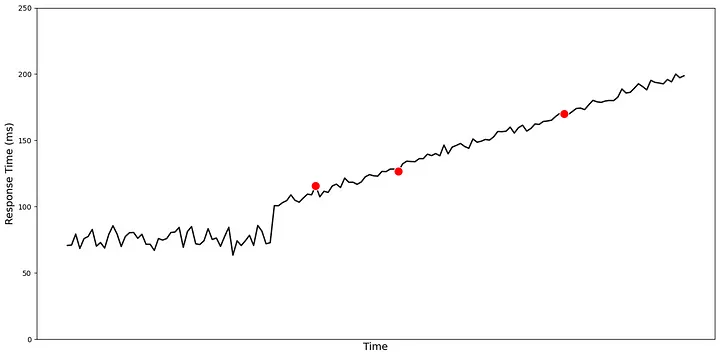
While point-in-time detection is effective for sudden deviations, it often falls short when the problem unfolds gradually. Metric data in real systems is inherently noisy — small fluctuations are common and expected. But what if a metric begins to drift slowly over time? If the change happens gradually and remains below configured thresholds, point-in-time detection will not raise any alerts. Yet, such patterns often precede real issues: a slow increase in memory usage, gradual degradation in application response time, or a queue that grows steadily without returning to baseline.
In these cases, the risk isn’t just a single spike, but a shift in how the system normally behaves. Sometimes, the average value of a metric starts to drift for a period of time — showing a temporary or evolving change from typical behavior. Other times, it’s not just the mean, but the distribution that changes — where the variance increases, or the shape of the data starts behaving differently. These variations may not be permanent, however they are important to detect and report as anomalies because they often precede real issues.
In many operational scenarios, we also observe trend changes, where a metric that was stable for weeks begins to exhibit a persistent upward slope. These transitions can occur linearly or in abrupt jumps from one regime to another. Both are difficult to detect without observing behavior over a longer window of time.
The challenge here is to distinguish between short-term noise and a true shift in the underlying signal. Raising alerts too early can lead to false positives and fatigue, while waiting too long risks missing early warning signs. Unlike point-in-time anomalies, which look at deviations from the recent past, span-of-time anomalies involve detecting persistent changes across segments of time. This means looking for shifts in patterns and trends — not in isolation, but in how the metric evolves over time.
To solve this, we begin by identifying key changes in the metric behavior — moments where the time series appears to transition from one phase to another. Once these points are identified, we evaluate whether the new segment of data behaves differently from the one before it. This difference could be in average value, variability, or slope. The goal isn’t just to detect that something has changed, but to determine whether the change is significant and meaningful in the operational context.
This helps surface anomalies that don’t appear as spikes but instead emerge gradually, shifting the system away from its baseline in subtle but important ways. These are often missed by threshold-based monitoring, and yet they play a major role in how issues develop over time.
Analyzing metrics in context: multivariate anomalies
Span-of-time detection helps identify gradual changes in individual metrics. However, real-world systems are rarely that simple. Most operational scenarios involve multiple interrelated metrics, and observing any one of them in isolation can often be misleading.
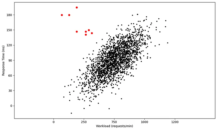
This is where multivariate anomaly detection becomes essential. Instead of analyzing metrics independently, we begin to evaluate how they behave in relation to each other. Metrics such as CPU usage, response time, transaction volume, queue length, and memory consumption are often closely connected — and changes in one are expected to influence others in specific, known ways.
Consider an example: an increase in workload typically leads to an increase in response time. This direct relationship is well understood, and by itself, neither metric may be anomalous. However, if workload remains steady and response time still rises, the relationship breaks — and that’s a signal worth paying attention to. Similarly, if request rates go up but queue lengths do not, we might infer that consumer throughput has improved; not that things are anomalous. However, if enqueue rates remain steady, but queue lengths start to increase, or if processing throughput drops unexpectedly, that’s when the usual relationship between metrics breaks — signaling a potential anomaly.
Identifying such relational shifts requires knowledge of which metrics are expected to move together, and in what direction. This often draws on domain knowledge or input from subject matter experts (SMEs), especially when interpreting behaviors tied to specific applications or infrastructure components. For example, the processing time of a batch job might depend on several factors: the number of files to process, the total file size, and the number of vCPUs allocated. Understanding these dependencies is key to interpreting whether a delay or queue buildup is anomalous or simply a result of expected workload changes.
Multivariate anomalies also help uncover indirect influencers — signals that may not show a clear anomaly themselves but help explain why another metric is behaving differently. This becomes important especially in diagnosing cascading issues, where the root cause lies upstream of the observed symptom.
By moving from single-metric detection to evaluating coordinated behavior across metrics, we gain a much richer and more accurate understanding of system health. It allows the anomaly detection system to filter out false alarms triggered by normal cause-effect relationships and focus attention on patterns that truly deviate from expected operational behavior.
Connecting the dots: composite anomalies
In complex systems, not all issues can be captured by looking at one metric — or even a group of related metrics. Many high-impact failures arise when multiple types of signals subtly drift within a short period; each may seem manageable in isolation, but together they point to a much deeper problem.
Composite anomalies refer to situations where different anomaly types — point-in-time, span-of-time, multivariate — occur across multiple sources such as metrics, logs, and events. They are often harder to detect, not because they’re hidden, but because no single signal crosses a critical line. Instead, it’s the coincidence of small shifts across different layers that creates the real risk.
Consider a system where:
- Memory usage has been steadily rising over several hours (a span-of-time anomaly).
- Response time is slightly higher than usual but still within tolerance (a multivariate deviation).
- And the logs show that the number of worker processes was recently scaled down (a configuration event).
Individually, none of these may trigger alerts. But together, they indicate early signs of system stress — possibly pointing to a memory leak combined with reduced processing capacity.
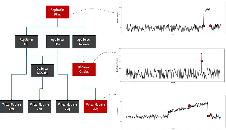
Composite anomalies are especially relevant in distributed systems, where different components may emit weak signals that don’t look critical until they are stitched together. They often reflect real-world failure modes, such as:
- Resource exhaustion across multiple tiers,
- Misconfigurations combined with load pattern shifts,
- Application slowdowns that correlate with infrastructure-level changes.
Detecting these requires a broader perspective — connecting dots across metrics, logs, and events. It’s not about looking deeper into any one metric, but about looking across metrics and identifying consistent, meaningful patterns that signal deviation.
Closing notes
Anomaly detection in modern IT systems is no longer about spotting a single outlier — it’s about understanding context, relationships, and evolving patterns. Point-in-time spikes, slow drifts, relational shifts across metrics, and subtle combinations of signals; all play a role in how real-world issues emerge and escalate. Relying on static thresholds or single-metric monitoring is not enough. Effective detection demands adaptive baselines, temporal awareness, and an ability to connect dots across the stack.
As enterprise environments grow more complex, the challenge isn’t just to catch what’s obvious, but to surface out the signals that matter — early, accurately, and with minimal noise. Ultimately, the goal is not just to alert, but to provide actionable insight — enabling teams to respond faster, prevent incidents, and maintain the reliability that today’s businesses demand.